Analyzing photo statistics using EXIF data

If you like photography and data analysis, you have probably wondered what focal lengths are more frequently used when shooting with your zoom lenses. Either by curiosity or to better inform your decisions on what lens to get next for your setup, it is definitely worth it to be mindful of what suits your style the most. Seeing your data explicitly plotted in a histogram might actually surprise you!

Fortunately, modern cameras imprint a lot of metadata into image files using a standard called EXIF, which stands for exchangeable image file format. Photo organization and processing software can retrieve such information using a powerful, yet simple and portable program called exiftool. We can take advantage of the features of this amazing software and write a script that can recursively retrieve image metadata from a database and plot it in a meaningful way.

I must disclaim that there is nothing super innovative about this approach. In fact, Yoke Keong posted a write up on the topic a decade ago, where they used exiftool combined with an R program to generate a histogram of their focal length usage. Proprietary software like Lightroom is also capable of displaying the data in a similar way. However, this feature is lacking on the most popular free software tools like Darktable, RawTherapee, and Digikam (as far as I know).

In my efforts to come up with a simple but versatile solution to plot my own data, I’ve found a convenient way to do that using more common tools. Below I share how to achieve interesting plots using Python and exiftool. Try it for yourself and the results might be surprising!

Creating the dataset, command line approach

If you would prefer to use Python exclusively and skip the command line entirely, jump to the PyExifTool section. Otherwise, keep reading.

Of course, the first step to analyze data is to create a dataset. For that, you can use the find command combined with exiftool to search for files and extract their metadata. This approach has been discussed elsewhere and in my experience, it works fantastically well.

Bottom line upfront, a simple one-liner command to recursively look for jpg images in a directory and gather focal length would be:

find . -name 'DSC_????.jpg' -exec exiftool -p '$FocalLength, $LensID' {} + 2>/dev/null | sort -n | uniq -c | sed -e 's/^ *//;s/ /,/' | tee ./focal-length-info.csv

Note that you might need to change 'DSC_????.jpg' to whatever formatting you or your camera uses for files, like 'IMG_????.JPG', or 'P???????.JPG', or whatever.

Now, we will break down what the command does. We first run find to look for files and execute a command on those files that were found. That is, find . -name 'DSC_????.jpg' -exec $command. The -exec option will execute the command that follows, and {} + will expand the matches.

In our case, this command will be exiftool. More explicitly, exiftool -p '$FocalLength, $LensID' {} + launches exiftool to look at the files found and prints $FocalLength and $LensID to stdout. The command (obviously) needs a file path as an argument, and {} + does exactly that, it sets the path as the matches of the find command. The purpose of 2>/dev/null is just to get rid of annoying warnings that might pop up.

We then pipe the stdout output to sort -n to sort by string numerical value (-n makes it such that integers are given a priority over strings, so 10 comes after 9). After that, uniq -c will count instances of repeated adjacent lines. The string separator of uniq is a space character, though. So to convert that to CSV, we pipe the output to sed -e 's/^ *//;s/ /, /', converting the first appearance of a space into a comma.

Finally, we pipe the output to tee, which will both show it to us in stdout and an output file. In our example, ./focal-length-info.csv. The file will look like this:

    167, 18.0 mm, AF-S DX VR Zoom-Nikkor 18-200mm f/3.5-5.6G IF-ED [II]
      1, 18.0 mm, AF-S DX VR Zoom-Nikkor 18-55mm f/3.5-5.6G
      9, 20.0 mm, AF-S DX VR Zoom-Nikkor 18-200mm f/3.5-5.6G IF-ED [II]
    ...
     14, 32.0 mm, AF-S DX VR Zoom-Nikkor 18-200mm f/3.5-5.6G IF-ED [II]
      1, 32.0 mm, AF-S DX VR Zoom-Nikkor 18-55mm f/3.5-5.6G
      5, 34.0 mm, AF-S DX VR Zoom-Nikkor 18-200mm f/3.5-5.6G IF-ED [II]
    ...
     17, 50.0 mm, AF-S DX VR Zoom-Nikkor 18-200mm f/3.5-5.6G IF-ED [II]
    239, 50.0 mm, AF-S Nikkor 50mm f/1.8G
     24, 52.0 mm, AF-S DX VR Zoom-Nikkor 18-200mm f/3.5-5.6G IF-ED [II]
    ...

Note: If you have read the original stack exchange answer I extracted this command from, you might be wondering why I added the LensID to it while the original answer doesn’t use it at all. Well, if you have a couple of prime lenses but want to analyze what zoom range you’ve been using the most, you can filter out the primes later on using some pattern matching.

Analyzing the dataset

After we have generated our dataset and exported it to focal-length-info.csv, it’s time to analyze it. The idea is very simple, just plot a histogram according to frequencies of focal lengths used. One problem might arise, though, which is the non-standard focal lengths when shooting with a zoom lens. For instance, 52 mm is virtually identical to 50 mm, so focal length extremities might be unfairly represented. For that reason, it might be a good idea to categorize the data into bins.

How you will exactly group and organize your bins isn’t an easy question to answer, unfortunately. It might depend on the format you shoot and what exactly you want to show. If you want to inform your next lens purchase, the best option is to just plot the focal length without converting them to full frame equivalent. If instead you want to compare your habits to those of professional photographers (or someone else) who quite likely shoot full frame, you can convert them to a full frame equivalent (by applying a crop factor) to analyze whether you are shooting wider or narrower than they are.

In my opinion, a good way of grouping focal ranges is following lens availability for your system of choice. For example, consider the diagram below for Nikon Z, showing their new lens roadmap (click to expand).

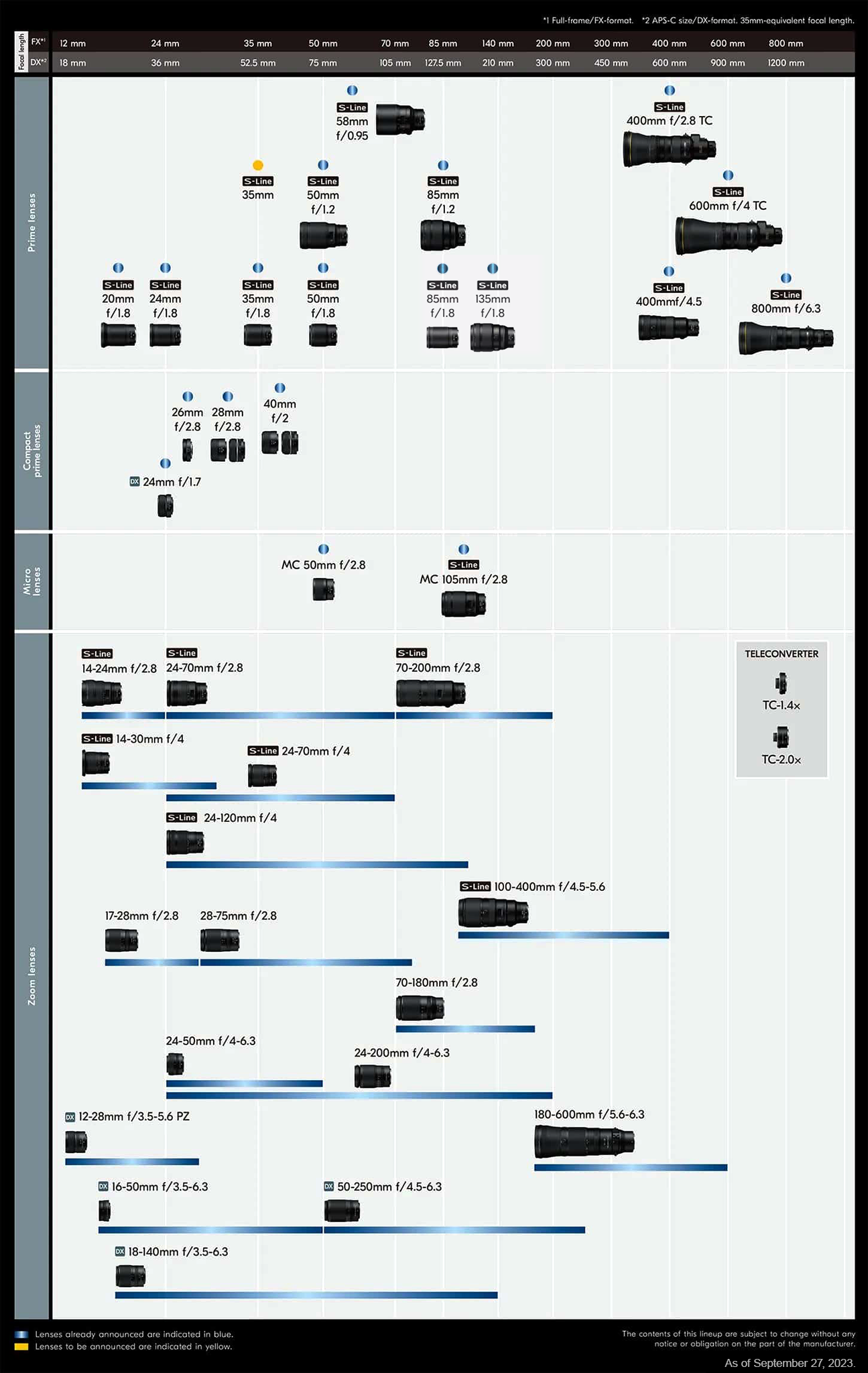Diagram showing Nikon Z roadmap, released by Nikon themselves. Click on the image to expand. Image posted in August 2023.

As you can see from the diagram above, lenses for Nikon Z full frame are:

Bright f/2.8 zooms (“holy trinity”): 14-24mm, 24-70mm, 70-200mm
Bright f/1.8 (or f/1.4) primes: 20mm, 24mm, 28mm, 35mm, 40mm 50mm, 85mm, 135mm
Lightweight f/4 zooms: 14-30mm, 24-70mm, 24-120mm
Do-it-all zooms: 24-120mm
Other zooms: 17-28mm, 28-75mm

If we are considering lenses for cropped sensors, there are extra options:

Zooms: 16-50mm, 24-50mm, 50-200mm
Do-it-all zooms: 24-200mm, 18-140mm

Then, a good way of organizing it in bins (in my opinion) is:

0-14mm, 14-16mm, 16-18mm, 18-20mm, 20-24mm, 24-28mm, 28-35mm, 35-50mm, 50-70mm, 70-85mm, 85-135mm, 135-200mm

For shorter focal lengths (wide angles), it is wise to consider 2mm spacing, since the field of view changes so much. For instance, in full frame terms, the field of view (FOV) of a 14mm lens is approximately 114 deg, while the FOV of a 16mm lens is ~107 deg. Just to put this into perspective, the difference between 150mm and 250mm is lower than that (7 deg). And we all know that 150mm and 250mm are very distinct fields of view already. If you are interested in the math, check out this link. Main point being, it is pointless to split 135mm and 140mm into two separate focal distances, since they are roughly similar, but worth it to split 14-16mm and 16-18mm into two separate bins. See the graph below for more details.

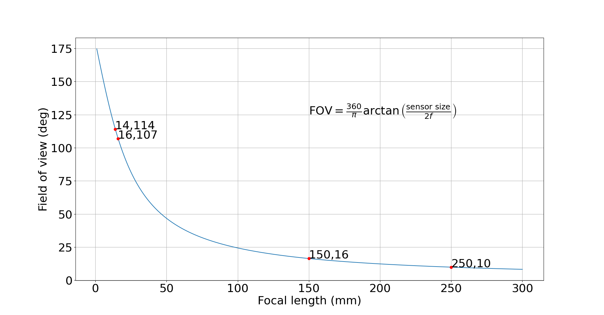Perspective formula and a plot of field of view (in degrees) versus focal length (in mm). Note how the difference in field of view between 14mm and 16mm is larger than the difference between 150mm and 250mm. Of course, we know that 150mm and 250mm are very different focal lengths, but this example is meant to illustrate how it is much more important to consider smaller changes in focal length for wide-angles than telephotos, since smaller changes will provide more dramatic changes in perspective.

If your system of choice is different, Wikipedia provides excellent pages on every major format, and you can check their tables as a reference to itemize your bins in a way that makes the most sense for you. The articles about Nikon F, Micro Four Thirds, Sony E, Fuji X, etc are all great.

Python

Now that we have covered the idea behind our analysis, let’s see how we can exactly approach this problem from an algorithm’s perspective.

# Define the bins you want to split your data into
bins = [0, 10, 18, 24, 28, 35, 50, 60, 70, 85, 105, 135, 150, 200, 300]
# Crop factor below.  Change it to 1.0 if shooting full frame or if you're
# not interested in converting your values.  Use 1.6 for Canon APS-C, 2.0 for MFT
crop_factor = 1.5

# If you want to limit your result to a specific lens,
# limit the analysis to zoom lenses, filter out a specific system, etc,
# add the filter here.
# It can be "Nikkor", "Zoom", "Olympus", "Sigma", etc.
filter_str = "AF-S DX VR Zoom-Nikkor 18-200mm f/3.5-5.6G IF-ED [II]"

Then, open the file and read all the entries

# Open the file to analyze the data, separate everything into a list
infile = "focal_lengths_with_lens_name.csv"
delimiter = "," # I'm using a comma here because I like CSV
with open(infile,"r") as f_in:
    splitted = []
    focal_lengths = []
    frequency = []
    # Organize the lists, for focal lengths, frequencies, and lens names
    for each_line in f_in:
        splitted = each_line.split(delimiter)
        # If you want to filter out a certain kind of lens, leave this here
        if filter_str in splitted[2]:
            focal_lengths.append(crop_factor*float(splitted[1].replace(" mm","")))
            frequency.append(int(splitted[0]))

Converting the lists to a dictionary makes it easier to work with later on. For that, I’m using Python’s zip approach

# Convert the lists to a dictionary
keys = focal_lengths
values = frequency
myDict = { k:v for (k,v) in zip(keys, values)}

Now that we have our Python dictionary, we need to count how many appearances were there in each bin that we defined before. It is a good idea to output the numbers in another CSV file, because we might want to analyze the raw data later, if a finer, more detailed inspection is required.

out_file = "binned_output.csv"
# Declare another dictionary which will contain the bins and frequency counts
freq_dict = {}
with open(out_file,"w") as fout:
    # For each focal length defined before, we want to check
    # what values are within such value and the next in the list
    for i in range(0,len(bins)-1):
        # For that, define a dummy variable "b" which will list all appearances/frequencies within that range
        b = { key: value for key, value in myDict.items() if bins[i] < key <= bins[i+1] }
        # Sum over all frequencies within the range
        sum_of_range = sum(b.values())
        # Print the value, write it to the file, add to the count
        print("The number of photos between "+str(bins[i]+1)+" and "+str(bins[i+1])+" is: "+str(sum_of_range))
        print("The (explicit) dataset is: ")
        print(b)
        print()
        bin_str = str(bins[i]+1)+"\n"+str(bins[i+1])
        fout.write(bin_str+delimiter+str(sum_of_range)+"\n")
        freq_dict[bin_str] = sum_of_range

If you want to plot a nice histogram using matplotlib, you can add the following to your code:

import matplotlib.pyplot as plt

plot_fname = 'output.png'
my_dpi = 96
plt.figure(figsize=(1366/my_dpi, 646/my_dpi), dpi=my_dpi)
bars = plt.bar(list(freq_dict.keys()), freq_dict.values(), color='g')
for bar in bars:
    yval = bar.get_height()
    plt.text(bar.get_x(), yval + 5, yval)
plt.title("Focal length statistics")
plt.ylabel("Shots kept")
plt.xlabel("Focal length (mm)")
plt.tight_layout()
plt.savefig(plot_fname, dpi=my_dpi)

The final file exported by matplotlib is shown below:

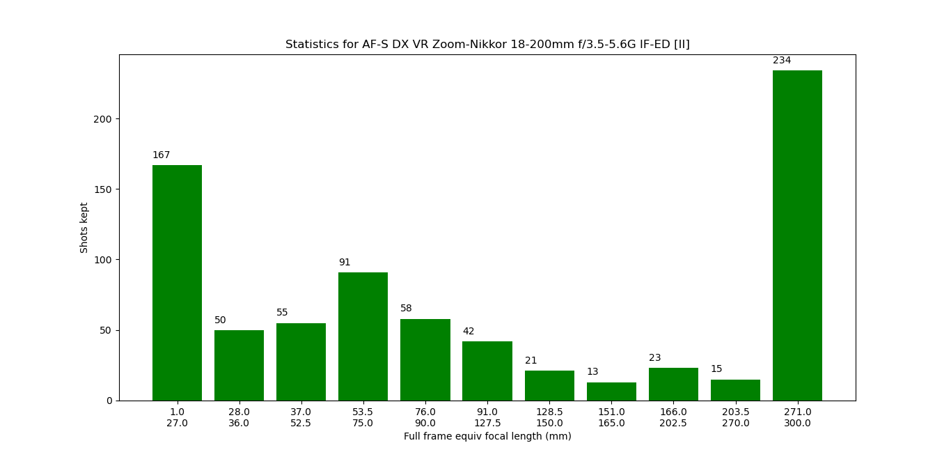Histogram showing a frequency of my "keepers" recently using the AF-S Nikkor 18-200mm f3.5-5.6 IF-ED II, as an output of the script I just shared. I was surprised to see how much I like the ~40~75mm perspective, and how relatively little I used the ~150~250mm field of view. Both the wide angle and telephoto extremities weren't a surprise to me, since I see myself wishing I had shorter or longer focal lengths quite frequently when using this lens. Notice that I plotted the focal lengths by applying the crop factor and thus converting to full frame equivalent.

Why any of this matters? Well, let’s consider a hypothetical scenario where I were to upgrade and get a Nikon Z FX (full frame mirrorless) or Nikon F FX (full frame DSLR) system and stick to zooms. By looking at the graph above, a good plan would be to consider saving enough to buy:

24-120 f/4 and 300mm f/4 (plus FTZ if using Z mount)
24-70mm f/4 and 70-200mm f/2.8 (with TC-2.0x or 1.4x, plus FTZ if using Z mount)
24-70mm f/4 and 70-300mm f/4.5-5.6 (Nikkor if Nikon F and Tamron if Nikon Z)

Any of those setups would be extremely versatile, cover most focal lengths I use, and produce fantastic images. Without looking at the histogram, I would guess I might miss a 200mm lens to fill the gap for option #1, but that wouldn’t be the case at all. With a smart approach to this, I could end up saving some money by skipping a 70-200mm f/2.8 plus a TC in favor of a prime 300mm f/4. Option #2 would then be out of question and the decision should be between #1 and #3.

PyExifTool

If you would like to restrict your usage to Python and not have to deal with the command line to generate the input file, there’s a tool called PyExifTool that got you covered.

First, we should import the exiftool module. Second, we want to generate a list with all the files we want to give to our algorithm. For that, we will use pathlib.

import exiftool
from pathlib import Path

# Create a list with all the input files
input_dir = "/home/user/Pictures/" # Change the directory accordingly
files = list(Path(input_dir).rglob("DSC_????.jpg"))

Don’t forget to change DSC_????.jpg to something that is relevant to you. Next, we want to create a blank dictionary and loop through all files in our list. For each file, we will extract focal length and lens ID. Just like we did before, if you want to filter out lenses, use the filter_str variable. If, for a certain image file, the lens ID matches what we are looking for, we will open the dictionary and add one to the frequency of that key (focal length).

# Leave filter_str empty if you don't want to filter out any lenses
filter_str = "AF-S DX VR Zoom-Nikkor 18-200mm f/3.5-5.6G IF-ED [II]"
# Crop factor below.  Change it to 1.0 if shooting full frame or if you're
# not interested in converting your values.  Use 1.6 for Canon APS-C, 2.0 for MFT
crop_factor = 1.5
myDict = {}
with exiftool.ExifToolHelper(common_args=None) as et:
    metadata = et.get_metadata(files)
    for d in metadata:
        LensID = d["LensID"]
        if filter_str in LensID:
            f = int(crop_factor*float(d["FocalLength"].replace(" mm","")))
            if f not in myDict:
                myDict[f] = 1
            else:
                myDict[f] += 1

print(myDict)

At this point you might be asking why use common_args=None, unlike the original example on PyExifTool’s pip page. That’s because PyExifTool includes the exiftool flags -G, -n by default. Thus, you need to add the common_args option so that both outputs match. This feature is documented here, and the same question has been asked before elsewhere.

At this point, we need to group all this data into bins, just like we did before.

# Define the bins you want to split your data into
bins = [0, 10, 18, 24, 28, 35, 50, 60, 70, 85, 105, 135, 150, 200, 300]
delimiter = ","
out_file = "binned_output.csv"
freq_dict = {} # Create an empty, binned dictionary
with open(out_file,"w") as fout:
    # For each focal length defined before, we want to check
    # what values are within such value and the next in the list
    for i in range(0,len(bins)-1):
        # For that, define a dummy variable "b" which will list all appearances/frequencies within that range
        b = { key: value for key, value in myDict.items() if bins[i] < key <= bins[i+1] }
        # Sum over all frequencies within the range
        sum_of_range = sum(b.values())
        # Print the value, write it to the file, add to the count
        print("The number of photos between "+str(bins[i]+1)+" and "+str(bins[i+1])+" is: "+str(sum_of_range))
        print("The (explicit) dataset is: ")
        print(b)
        print()
        bin_str = str(bins[i]+1)+"\n"+str(bins[i+1])
        fout.write(bin_str+delimiter+str(sum_of_range)+"\n")
        freq_dict[bin_str] = sum_of_range

Now that all the hard work is complete, we just need to plot the graph exactly as we did before! Copy and paste the code below and voila, you have the same matplotlib output you were to get using the exiftool command line tool piped to a CSV file.

lens_name = filter_str
my_dpi = 96
plt.figure(figsize=(1366/my_dpi, 646/my_dpi), dpi=my_dpi)
bars = plt.bar(list(freq_dict.keys()), freq_dict.values(), color='g')
for bar in bars:
    yval = bar.get_height()
    plt.text(bar.get_x(), yval + 5, yval)
plt.title("Statistics for "+lens_name)
plt.ylabel("Shots kept")
#plt.xlabel("Full frame equiv focal length (mm)")
#plt.xlabel("Focal length in cropped (mm)")
plt.xlabel("Focal length (mm)")
plt.tight_layout()
plt.savefig('output.png', dpi=my_dpi)

And there you go! A script written in Python that can do exactly what we have done before, without any need for explicitly using the exiftool on a terminal emulator.

Webpage

It would be awesome if there was a web page where you could upload the CSV data file and then see nice plots using a beautiful data visualization library. I will work on putting something together and publish it here, and perhaps a GTK application using PyExifTool to do the same.

Creating the dataset, command line approach

Analyzing the dataset

Python

PyExifTool

Webpage

Useful links and references